Category: Uncategorized

We got a bit of functionality to show. There is now a github repository. https://github.com/lennart-benschop/term_bitmap. The library works in the Linux terminal and it is 13kB in size. It can be statically linked against your own programs to allow them to draw graphs in a Linux terminal.

It can draw graphs in terminals in the following ways:

• Sixel protocol: supported by the original xterm, but also by KDE Konsole, Wezterm, foot and some other modern terminals.
• Kitty protocol: supported by kitty, ghostty and some other modern terminals.
• Linux framebuffer: supported by the Linux console outside the graphical desktop.

Apart from this, it can draw character-based graphics using sextants, octants and braille characters, all in monochrome. These have a much lower resolution than the true graphics modes, but they work on more terminals.

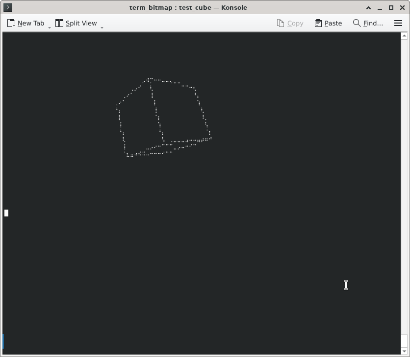
A spinning cube (wire outline) using braille characters looks like this::

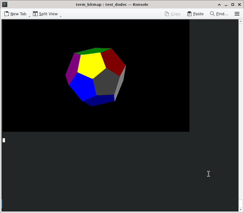
Using sixels, a spinning dodecahedron with solid coloured polygons looks like this:

Architecture.

The library revolves around the tbm_bitmap_t data structure. This contains essential parameters of the bitmap, such as width, height, palette, graphics drawing protocol and of course a reference to the bitmap itself. The bitmap is an array of bytes, one per pixel, allowing for a maximum of 256 colours.. The data structure and the bitmap are not exposed to the public API (which uses void pointers to as references to it). All access to the data structure is through API functions.

For each drawing protocol, there is one tbm_out_*.c file, that contains a redraw function and a function to constrain bitmap sizes (for sixels we ensure the height is a multiple of six) and colour depths. The tbm_main.c file contains two switch statements that control the polymorphism.

The drawing protocol to use us mainly determined by the environment variable TBM_MODE. If this is not set, the TERM variable is used instead. However, many terminal emulators just provide xterm-256color in this variable, making it not very practical to find out what is actually supported. Therefore, in most cases the user must set the TBM_MODE variable.

A program using the library will typically call tbm_get_recommended() first, which provides a recommended drawing protocol and estimates of the resolution and colour depth supported. This function checks the TBM_MODE and TERM variables as described above. Using the parameters just obtained, it calls tbm_new_screen(), to create an empty bitmap. The function tbm_redraw() will actually show the bitmap on the screen.

The functions tbm_plotdot(), tbm_lineto(), tbm_triangle(), tbm_circle() and tbm_plottext() actually draw things into the bitmap. Any updates will not be visible until tbm_redraw() is called. Animations are possible, including simple games, like we did on the old 8-bit machines.

FORTH

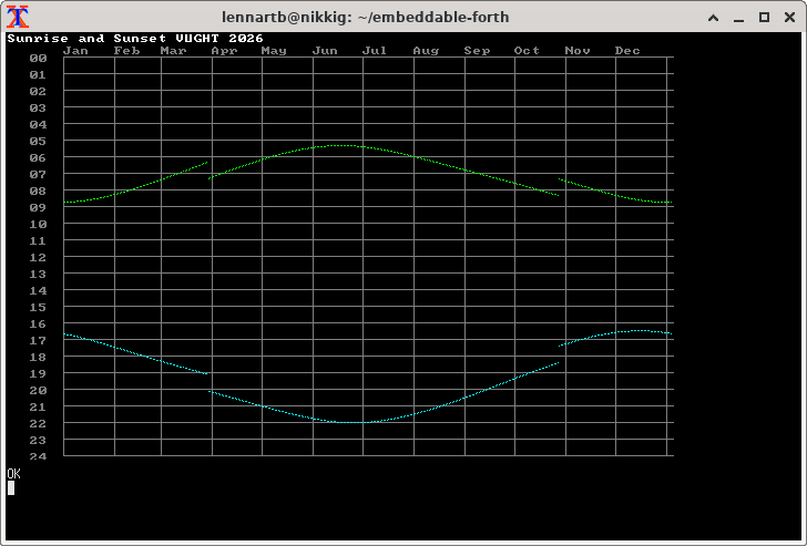
One of the programs that links with our new library is my embeddable FORTH. https://github.com/lennart-benschop/embeddable-forth. It can now draw graphics interactively. I ported a few programs from Agon FORTH. The below picture shows a graph of sunrise and sunset times over the year 2026:

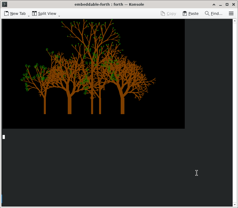
The picture below shows some trees being drawn algorithmically, also in FORTH:

Back in the early 1980s, most home computers came with BASIC in ROM. As soon as you switched the machine on, you were invited to write a program. Programming was easier to access than anything else on the machine. On many such machines it was also trivially simple to draw shapes on the screen. From simple lines, you could create triangles circles and more complex patterns, all using a few lines of BASIC. You discovered how to draw a graph of some mathematical function on the screen. When you made a mistake, you saw immediately what went wrong. This was interactive programming at its best.

If you happened to have a Commodore 64, you were not so lucky. BASIC did not support graphics commands and you needed to type a lot of pokes, just to get the VIC chip into graphics mode (at which time you could no longer read the normal text). Other machines, like the ZX Spectrum and the Acorn Electron really invited you to draw on the screen.

Acorn (BBC Micro, Electron, Archimedes, RiscPC)) added graphics support to the terminal driver. This way you could plot dots, lines and triangles by sending bytes to standard output. This was accessible to all programs, not just to BASIC. The Acorn terminal command set contains some pretty advanced features: you can set both a text and a graphics viewport and text or graphics output remains confined to the specified area (text even scrolls within that area). You can scroll in all directions and you can even redefine the bit patterns of the characters.

Unix terminals

When UNIX was introduced, terminals were still printing teletypes that could print only text. Interactively changing the text in the middle of the page just was not a thing. Some early video terminals could only add text to the bottom row and scrolled everyhing up, without any way to control the cursor. But that changed rather quickly and before long we had terminals that were capable of positioning the cursor anywhere on the screen and editors like vi could be implemented. It as all exclusively ASCII text though.

In the early 1980s we got some terminals that could display graphics. Some DEC terminals could display bitmaps using the sixel protocol. In this protocol, a column of six pixels is represented by a single character. Send many characters and you get a row if bitmap graphics, six pixels tall. It works the same way as some printers could draw graphics. At 9600 baud this was not particularly fast. No flashy games were possible. But you could prepare a high resolution bitmap of a diagram of graph and show that on the screen.

Some DEC terminals additionally had support for ReGIS (Remote Graphics Instruction Set). You could plot lines and circles etc. using simple commands. This is the closest to what Acorns VDU driver has to offer, but it was only available on very few terminals. Support of it died out rapidly. Of the modern Unix terminal emulators, only xterm supports it, but it is a compile-time feature that has to be specifically enabled and most distributions do not enable it (sixel support will typically be supported by default). For all practical purposes, ReGIS is dead.

Terminals with some graphics support gave way to X Terminals, which require a very complex software stack to be used.

Linux (and other PC Unix-like systems) tried to replicate what was available on typical Unix machines, not what contemporary PC hardware could support. Terminal drivers in Linux would replicate the vt220 command set (sort of), but no sixel support, let alone ReGIS. And of course X was available. But in order to make a program draw some lines in X, you have to learn a lot of APIs to make it possible and your application will now be a GUI application with an event loop, not a straightforward command line application that happens to draw some lines.

Modern Linux

Terminals in modern Linux do support drawing bitmap graphics, but there are at least three ways to do it:

• Sixel support, like the old DEC terminals could do. This is still supported in Xterm, but also in some other terminals, like Konsole on KDE.
• The Kitty protocol. This is supported by the kitty terminal, but it is also implemented in other modern terminals like Konsole and ghostty.
• The Framebuffer device, that can be used in the Linux console (when not running a GUI).

Data transfer using the Sixel protocol is now several orders of magnitude faster than it was in the 1980s, so now it is a totally practical way to render interactive games inside the terminal. Kitty and framebuffer can do this as well.

But some frequently used terminals, such as the GNOME terminal, do not support bitmap graphics at all. But all is not lost. Unicode supports symbols for legacy computing. There are several sets of symbols:

• The sextants, characters that consist of a matrix of 2×3 pixels. Characters like this were found on the TRS-80, the Mattel Aquarius and in Teletext. A 80×24 screen could show 160×72 blocks this way. Unicode fonts are unlikely to contain these characters, but many terminals (like the GNOME terminal) have dedicated support to show these. Konsole and Kitty also do a good job (but they have proper bitmap graphics as well).
• The octants, characters that consist of a matrix of 2×4 pixels A 80×24 screen could show 160×96 blocks this way. These are a fairly recent addition and are not well supported by many terminals. The Gnome terminal does support these. Interestingly enough, Kitty supports the characters in the dedicated octants range, but fails to render several characters that got defined in other ranges because they define the same block pattern.
• The braille patterns. Unicode contains a full set of 2×4 braille patterns, mostly shown as a rectangle of dots. However, these are not shown as a contiguous pattern of dots, you keep seeing the 2×4 blocks. But these are supported nearly everywhere. Much uglier than octants, but more widely supported.

In a typical Linux GUI, we can stretch a terminal window up to 160×80 characters (especially using a small font). and this allows us to get 320×240 bitmaps using sextants. This is usable for displaying photos and it is even possible to show video. With all these character based solutions, each character cell can contain only one foreground and one background colour, so there is some colour clash.

There is a library called notcurses https://github.com/dankamongmen/notcurses that can show bitmaps in a terminal using all protocols mentioned so far. But this is a rather heavyweight library and it is focused on showing bitmaps, not on simple line drawing.

Terminal Bitmap Library

Right now I am developing a lightweight library in C that can draw lines, pixels and text (and will add triangles and circles) using simple function calls. I started a github project https://github.com/lennart-benschop/term_bitmap No stuff is there yet, but that can change. The intention is that we can link this to a FORTH or BASIC interpreter and get easy line drawing from these.

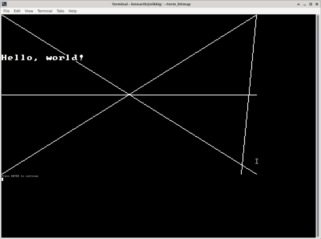
Below is an Xfce4 terminal, stretched to more than 160 chars wide and more than 50 chars tall (tiny font), showing a 320×200 bitmap using octants. Only monochrome is supported right now.

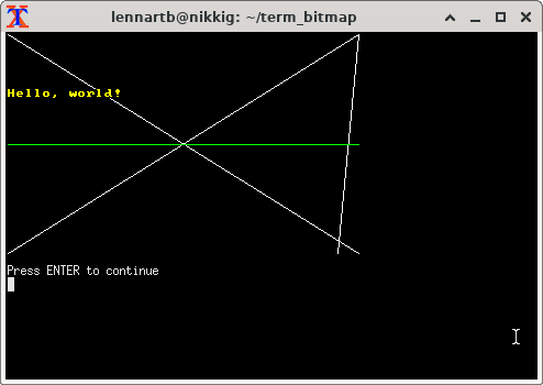
Here is the same image rendered using sixels in xterm and now in colour.

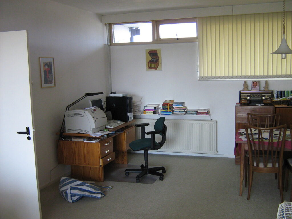
In 2007 I lived in an apartment in Eindhoven. This photograph is from the living room. My main computer was on the wooden desk on on the left side of the picture.

On the left side of that desk, there is a big laser printer, I think it was a Lexmark. I bought it back in 2003 on the used market. A new toner cartridge cost more than the printer itself. The monitor is a Philips 19” LCD screen, that I still have. There was an old IBM heavy keyboard. The black tower case was the main computer, a Core 2 Duo, that I bought in the autumn of 2006. Originally it had only 1 GB of RAM, later it got 4. The white box on top I got as surplus material from my employer. With some hacked together Linux software, it acted as an NAT router. Cable internet allowed you to connect one device at that time. Cable modems did not yet include their own built-in NAT routers as later models would have.

I had a fancy sound card and a DVD burner, that I used regularly to burn CDs. And I ran 64-bit Linx: the Gentoo distribution.

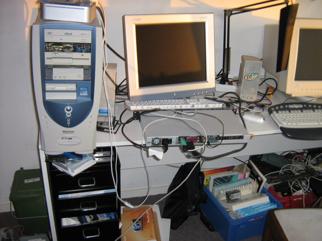
The other photograph is from my larger bedroom (the spare room). I used my smaller bedroom for sleeping.

On the left we see a large Mycom branded (one of the larger computer stores in the Netherlands) tower case. It had a DVD ROM drive (only a reader, the writer was in the main PC). Below that, there was a 5.25” floppy driver that I salvaged from an older PC. Below that we see a SCSI tape drive and finally we have a 3.5” floppy drive. I purchased the machine originally in the autumn of 2003, a Pentium 4 with 512 MB of RAM. It was hyperthreading, but not a true dual core. On top if this we see a Mac Mini, the original one from 2005, PowerPC-based with just 256 MB of RAM. Both of these machines ran Gentoo Linux. The PC dual booted with Windows XP and the Mac dual booted with OS-X (the PC in the living room was Linux only). To the right of this PC we see a Liteon 17” LCD monitor and the Apple keyboard. Both were used with the MAC Mini.

The metal box below that Apple keyboard was an “industrial PC” with a Via EPIA board. It ran Debian and I occasionally used it for unattended recording of radio programmes. I had to hook up a radio to the audio input for that. To the right we see a Microsoft keyboard and a 17” CRT monitor. Both were used with the PC on the left and occasionally with the VIA EPIA machine.

The original Intel 8087 supported an 80-bit floating point format with 64 bits of mantissa and 15 exponent bits. This is more than the double-precision format of IEEE-754. This 8087 architecture is still with us in modern Intel and AMD CPUs, even though it is largely overtaken by the SSE2 extension that supports only regular single and double precision floating point numbers. The 80-bit extended precision float format is slower than the modern SSE2 instructions, but it is still available to C programs.

Other widely available CPUs, such as ARM and RISC-V do not have this extended precision format at all. RISC-V defines a full 128-bit quad-precision floating point extension, but the number of CPUs that actually implement this in hardware is zero. POWER-9 and IBM zSystem CPUs do implement 128-bit quad precision in hardware, plus decimal floating point. These are not in your regular desktop PC of phone.

For all practical purposes, 64-bit double-precision is enough. The 53 bits of precision are enough to express the length of a trip to Mars to within one millimetre. That said, modern atomic clocks reach a precision of 10^-14, getting somewhat close to the 15-digit precision our double floating point numbers have. Extended precision may be useful for providing maximally precise implementations of logarithmic and trigonometric functions for programs using double precision. The round-off errors that occur when computing these functions in extended precision, disappear in double precision. Of course there is number theory study. It is super important to know the statistical distribution of digits of Pi. 128-bit floating point does not cut that either and we use arbitrary-precision libraries for it.Pi has been computed to a several trillion digits (10¹² ). Therefore the use of 128-bit floating point is rather limited and

With the old Intel CPUs, single-precision and double-precision did not compute any faster than 80-bit extended precision. The 32-bit single and 64-bit double floating point formats were just storage formats, the 80×87 computed everything in extended precision anyway. The downside was, that programmers in high-level languages had no idea how and when the compiler stored intermediate results into memory (thereby rounding them) and when it kept them in internal registers, keeping the full precision.

The original C standard even specified that intermediate results had to be double precision, restricting the use of faster 32-bit single precision operations on CPUs on which these were indeed faster.

When doing large numerical operations, like linear equation solving and numerical integration, round-off errors add up. You may lose several digits of precision. Single-precision may not be enough for some applications. If you start with 7 digits and end with just 3 digits of precision. But in many cases, even 3 digits of precision of the end result, is just enough. Some microcontrollers. like the ARM Cortex-M33, have only single-precision floating point support, no double precision in hardware. If you can get the job done with just single precision, it makes the difference between a viable system or not. On modern CPUs with SIMD or vector hardware, throughput of single precision operations is at least twice that of double precision, just because you can do twice as many operations in parallel.

Enter the world of 3D rendering. Pixel values can have a high dynamic range, maybe 1 to 1 billion or more. 16-bit floating point numbers offer a dynamic range greater than 32-bit integers, but requiring half the bandwidth. The half-precision format has 5 bits of exponent and 11 bits of mantissa (implicit leading one). Modern CPUs offer half-precision floating point numbers, twice as many in parallel as single-precision numbers. GPUs (Graphics Processing Units) are typically built around half-precision floating point numbers.

Machine learning is another field that benefits from small floating point numbers. Half-precision floats are well suited for it. Coefficients of a neural network require a rather large dynamic range, but low precision. Once a model has been trained, its precision can be reduced even further to 8 bits or 4 bits.

The digital telephone network has been around since the 1970s. It uses 8-bit audio samples at a sampling rate of 8000 samples per second. Therefore it is 64kilobits/s. The samples are not linear PCM, but a format with a higher dynamic range with less precision for higher values and more precision for lower values. This is called A-law or µ-law curve. This is very similar to an 8-bit floating point format. The dynamic range of the raw samples is 13 bits (A-law) or 14 bits (µ-law), but they are compressed into 8 bits. Both A-law and µ-law curves are in use.

Come to think about it: a four-bit floating point number can have 16 distinct values. Typically they are -6.0, -4.0, -3.0, -2.0, -1.5, -1.0, -0.5, -0.0, +0.0,. 0.5, 1.,0, 1.5. 2.0. 3.0, 4.0 and 6.0. The ratio between the largest value (6.0) and the lowest non-zero value (0.5) is just 12. For 4-bit integers this would be 7. Four-bit floats skip the infinity and NaN values (but is is possible to replace -0.0 with a catch-all for infinity and NaN).. Four-bit floats are used in Large-Language models, not for training purposes but to store them once they are trained. They are often stored in groups, with an additional scaling factor per group.

8-bit and 4-bit floating point numbers are also sometimes used for education, to illustrate how IEEE-754 works. A four-bit floating point format is the minimum that has all the important elements. The 16 values would now be. -NaN, -Inf, -3.0, -2.0, -1.5. -1.0, -0.5, -0.0, +0.0, 0.5, 1.0, 1.5, 2.0. 3.0, +Inf and NaN. We can show the results of operations like addition, subtraction, multiplication and division in single-page tables, for each of the four rounding modes. The 4-bit float has one sign bit, two exponent bits and 1 mantissa bit, giving 2 bits of precision using an implicit leading 1.

Even though, IEEE-754 is a huge improvement compared to the floating point implementations that existed before, it still has many counter-intuitive properties.

0.1 is a repeating fraction.

In binary integers, each bit represents a power of two, like 2⁰, 2¹, 2², etc. For example the binary number 1011 (read the digits from right to left) is equal to 1×2⁰ + 1×2¹ + 0×2² + 1×2³ =1 + 2 + 8 = 11 in decimal. Binary fractions have digits to the right of the binary point. These digits to the right represent values 2^-1, 2^-2, 2^-3… etc, which means ${1 \over 2}$, ${1 \over 4}$, ${1\over 8}$, … Thus, the digits after the binary point do not represent ${1 \over 10}$ or ${1 \over 100}$. With binary fractions, we can exactly represent fractions like ${5 \over 8}$ or ${7 \over 32}$ but not ${1 \over 10}$.

The binary fraction for ${1 \over 10}$ is 0.00011001100110011001100….. This is an infinitely repeating fraction, just like with decimal fractions the number ${1 \over 3}$is 0.333333…. No matter how many decimal places you have, it will never be exact.

For engineering applications this does not matter much. All measured and computed values are approximations of the real value anyway and floating point numbers are nearly always accurate enough. For accounting, this is a different story. We want the exact same totals on both sides of the balance sheet. And when we represent amounts with floating point numbers in a straightforward way (£1.36 is represented by the floating point number 1.36), we are not going to get it.

Real accounting programs should use integer maths (and using large integers of 64 bits or preferably 128 bits at that). Amounts are integers and percentages are computed with integer arithmetic and rounded correctly at each division by 100 or by 1000. Many people use spreadsheet programs to do their accounting and spreadsheets may or may not use decimal arithmetic when they think a column represents monetary amounts. Spreadsheets usually contain too many bugs to be taken seriously for these applications anyway.

It gets even worse when floating point computations are used to determine control flow. BASIC allowed you to index loops with floating point values. In the program below, it is not clear whether the loop will include the value 2.0 or not.

10 FOR A=0.1 TO 2.0 STEP 0.1
20 PRINT A
30 NEXT A

There is no problem, however if you use floating point values that are exactly representable. The loop below can be counted on to include the value 2.0.

10 FOR A=0.125 TO 2.0 STEP 0.125
20 PRINT A
30 NEXT A

There do exist decimal floating point libraries that represent decimal fractions exactly like you would expect and that can do decimal computations with exact results and correct rounding. Some CPU architectures (Power 9) implement decimal floating point in hardware, but this is not the case with x86, ARM or RISC-V.

Addition is not associative

Try to type the following lines of code in Python (similar code works in any programming language using floating point):

a = (0.1+0.2)+0.3
b = 0.1+(0.2+0.3)
print(a-b)

As you see, the values a and b are not equal! Whenever a floating point result is not mathematically exact, there is a chance that the final result depends on the way you group the operands.

The difference may be tiny in this case, but if the values have wildly different magnitudes and both positive and negative values are involved, the difference can be crucial. These are special algorithms to sum a large number of numbers in such a way that the output is as close to the correct answer as humanely possible.

Compilers should not rearrange floating point operations in an expression and they should not optimise away seemingly redundant operations. Those seemingly redundant operations may be there to implement a special trick to obtain a more accurate result than without them,

NaN is a weird thing

When you try to divide a positive number by zero, you get +infiinity as a result, when you divide a negative number by zero, you get -infinity instead. The same +infinity or -infinity can also result from ordinary overflow. When you divide 0 by 0, you get NaN, which means Not a Number. NaN would also result from subtracting infinity from infinity for example and in some other cases where the operation was clearly invalid. Every arithmetic operation you perform with one or both operands NaN, will result in NaN as well.

In a large simulation, some points in space may end up with a NaN value, while most of the space may still contain useful values. This is the reason why NaN results are propagated instead of stopping the whole simulation on an invalid operation.

NaN has some counter-intuitive properties:

• Every comparison against NaN will give a false result (except for the isNaN predicate). Therefore, if A is NaN, A<0 will be false, but A>=0 will be false too. A==A will even be false.
• When the MAX or MIN functions are used with one NaN and one proper number, the proper number is returned. This is one case, where NaN is not propagated if one operand is NaN

Rounding modes

Error analysis of floating point algorithms is hard. so hard that most programmers don’t even try to do it at all, let alone do it properly.

Rounding modes can be used to perform a crude form of error analysis. The IEEE-754 standard requires each implementation to support four rounding modes: round to -infinity, round to 0, round to +infinity and round to nearest. You can run the exact same computation in all four rounding modes and compare the results. The number of significant bits that agree in all four results, is a useful measure of the rounding errors in your computation. The more bits agree in all four results, the more reliable the result is. This is not bulletproof, but better than nothing.

There are cases where all precision is lost and the computed result is exactly zero, regardless of the rounding mode. However, the result should not have been zero. Comparing the results in different rounding modes, will not find the problem in this case.